
Using the Query view
So far we've looked at the database at rest. The Query view watches what the storage engine actually does when a query runs - it traces the query and replays the activity on a timeline.
This section of the tutorial covers:
- Using the Query view - executing a query with a trace and reading the timeline
- Views and layout - the panes and how to arrange them
- The execution plan - the plan connected to the timeline
- Scans vs seeks - the two fundamental access patterns compared
- Lookups - key lookups, covering indexes, and RID lookups
- Joins - the three physical join operators and their access patterns
- Log Records - tracing a delete down to the byte level
It uses the dbo.ClusteredTable table and IX_ClusteredTable_TextField index created in Parts 2 and 3.
Open the Query view
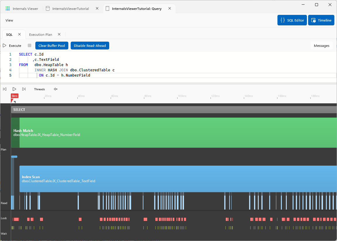
Click the Query button on the database toolbar. This opens a Query tab for the connected database with a SQL editor.
Execute a query
Enter a query and press Execute:
SELECT Id
      ,TextField
FROM   dbo.ClusteredTable
WHERE  TextField LIKE 'This is row 123%'
Internals Viewer runs the query with a trace session and captures what the engine did - physical page reads, locks acquired and released, waits, page splits, the execution plan, and more. When the query completes the captured activity is loaded into the timeline at the bottom.
Clear Buffer Pool and Disable Read-Ahead on the editor's command bar make this activity more visible - see SQL Editor for what they do.
NOTE
Data modification queries (INSERT / UPDATE / DELETE) are run inside a transaction that is rolled back after the trace is captured, so you can experiment without permanently changing the data.
The timeline
The timeline at the bottom shows the captured activity against time, replayed with playback controls - play, step, speed, and a draggable playhead. See Timeline for the full set of bands and how to work with it.
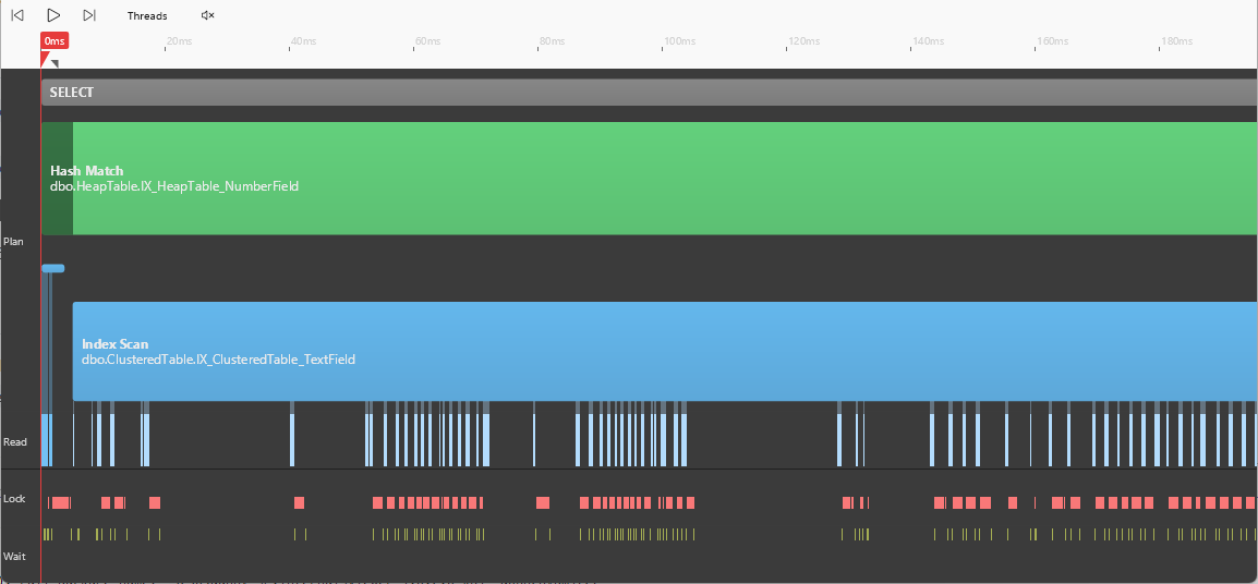
Zoom in on the Read band - each tick is a single 8 KB page being read from disk. For our indexed query there should only be a handful of reads: the root-to-leaf seek we walked manually in Part 3. Now try a query that can't use the index:
SELECT Id
      ,TextField
FROM   dbo.ClusteredTable
WHERE  TextField LIKE '%row 123%'
The leading wildcard forces a scan, and the Read lane fills with page reads as the engine works through the whole table. Scans vs seeks digs into this contrast.
Operators and the iterator model
The bars in the Plan lane make more sense with a picture of how a plan actually executes. An execution plan is a tree of iterators: execution starts at the top, and each operator asks the operator below it for a row, which asks the operator below it, and so on down to the operator reading pages. Rows are pulled up through the tree one at a time - the SELECT at the top pulls a row, and a chain of requests ripples down and a row ripples back up. An operator's bar in the Plan lane spans the time it was active in this process.
How an operator responds to that pull is what divides them into two kinds:
- Streaming operators hand each row on as soon as they receive it. A scan, a seek, a Compute Scalar, a Nested Loops join - rows flow through them continuously from the first request.
- Blocking operators can't produce their first row until they have consumed their entire input. A Sort is the clearest example: it can't emit the first row (the smallest value) until it has seen the last input row, because the last row might be the smallest.
Clicking an operator's bar in the timeline selects it and highlights when it actually streamed rows. Try a query that has to sort:
SELECT NumberField
      ,TextField
FROM   dbo.HeapTable
ORDER  BY TextField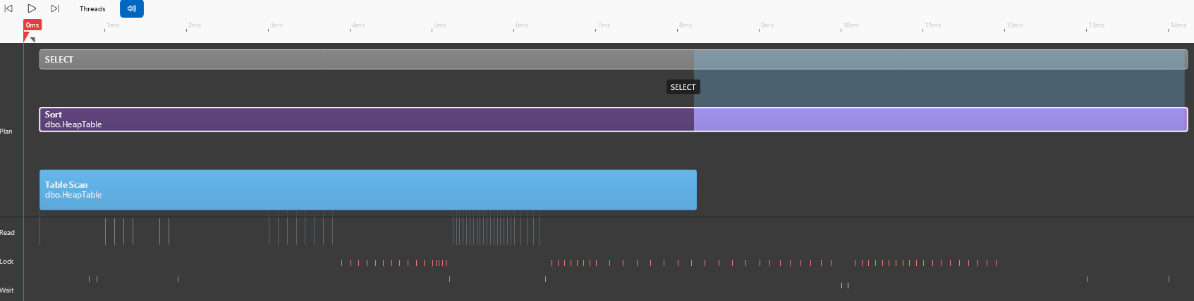
Click the Sort's bar: for almost its whole lifetime it is consuming its input - pulling every row up from the scan below - and only at the very end does it stream its output to the SELECT above. The gap between "active" and "streaming" is the blocking behaviour made visible. Compare it with the scan feeding it, which streams for its entire bar.
This distinction runs through the rest of this section - it is why a hash join has two phases, and why one blocking operator low in a plan delays everything above it.
Next: Views and layout