Trace Timeline

The Trace Timeline draws every call recorded by a Full Trace - one lane per thread, one bar per call, each call nested beneath the call that made it. The bars use the Call Tree's category colours.

The Call Tree merges every call down the same path into one row with a count. The Trace Timeline keeps each call apart, in the order it happened, so a scan's GetRow calls show as a run of short bars, one per row, and a function called once for a long time as a single wide one. It takes the Timeline's place while Record Full Trace is on, and the Trace Timeline item on the View menu, enabled only then, brings it back if it is closed.

Reading the chart

From top to bottom:

• The ruler - how far through the recording, in trace positions or instructions - see Position and instructions. Click it to put down the playhead
• The Operators pane - with Operators on, a row per plan operator - see Operators
• The Memory History lane - with Memory on, the memory blocks the query wrote to and the writes to each
• A lane per thread - headed Thread and the operating system thread id
• The memory band - with a view chosen under View > Flame Chart > Memory, the memory allocated and in use along the bottom - see Memory

Operators, Memory and Calls on the tab strip show and hide the Operators pane, the Memory History lane and the thread lanes. The last of the three left on cannot be turned off. View > Flame Chart > Highlight Regions shades the stretches of the lanes where the query was compiled, started and shut down, as Compilation, Setup and Shutdown, each with its own toggle. View > Memory History > Writes and Reads, also on the lane's right-click menu, choose what the lane marks: writes, which are on by default, reads, or both. A read is marked once for each call that read a block, at the position of its first read and across the bytes it read, in a lighter shade of the reading call's category colour. The lane also holds the objects a function keeps on its own stack once it hands them to another function, as the object a member function is called on, or as an argument or return value declared as a pointer to a class. Such an object is read as it is handed over and again when that call returns, so its changes are what was different at each handover, credited to the function handing it over or to the function it was handed to. A function's local is one object however often the function runs, and each call is an instance of it, so the lane draws a bar for each call and its changes run on from one call to the next. Clicking one moves the playhead there and opens the block. View > Memory History > Size to Fit, on by default, squeezes every block into the lane. Turn it off to draw the blocks at their relative sizes, with a scroll bar always on the right of the lane, and the mouse wheel over the lane scrolls through them. View > Memory History > Call Highlight Hover dims every call except the ones that wrote to the block under the pointer while you hover over the Memory History lane. View > Memory History > Latching and BUF are covered in Buffer latches. View > Reset Layout puts the pane heights back and docks the Call Stack and memory tabs beneath the chart again. Right-clicking any of the three areas offers the same three toggles, with the only area still showing greyed out, then that area's own view settings and Call Stack, so the View menu's settings are a click away wherever you are. Right-clicking a block in the Memory History lane also offers Open Reference Graph for that block, covered under Call Stack.

In a lane, each call is a bar running from where it started to where it ended. The calls it made sit directly beneath it, inside its width, so the outermost call is at the top of the lane and each row down is one level deeper in the stack. That is the reverse of a classic flame graph, which grows upwards, but it reads the same way as the Call Tree. A bar is coloured by its function's category and labelled with the function's name once it is wide enough to read.

• A wide bar - a call that ran for a long stretch, and on the Instructions axis, one that executed a lot of code
• A run of thin bars - the same function called over and over, such as a scan's GetRow once per row
• A gap beneath a bar - the call working in its own code rather than in a call it made, or in Extended Events and tracing code, which is left out of the chart
• A pale strip - calls too narrow to draw one by one, merged into a single strip. Zoom in to pull them apart

The Trace Timeline is not the Flame Graph on the Execution Plan, which breaks each operator's bar down into the calls sampled from its events.

Position and instructions

TTD has no clock. A recording is a sequence of positions - a sequence number shared by every thread, plus the number of instructions the thread has executed since - so the ruler is never in milliseconds. View > Scale chooses what a bar's width means:

• Position - the default. Width is the span of trace positions a call covered. Positions are shared by every thread, so the lanes line up against each other and parallel workers can be compared. A position moves on by one whole step at each point where a thread synchronises with another or leaves the recorded code, however many instructions came before it. So short calls that cross one of those points come out about the same width, and calls that stay inside the recorded code without crossing one are thin.
• Instructions - width is the number of x64 machine instructions the call executed, including the calls beneath it, which is the closest the recording has to how long a call took. Only the storage engine and query processor are recorded, so time spent in SQLOS or Windows - allocating memory, waiting, reading from disk - adds next to nothing. Each thread counts its own instructions from zero, so every lane starts at the left and the lanes do not line up.

Moving around

• Mouse wheel zooms in and out at the pointer
• Shift + mouse wheel, or a horizontal wheel, pans sideways
• Ctrl + mouse wheel scrolls through the threads
• With Size to Fit off, the Memory History lane keeps a scroll bar on its right, the mouse wheel over the lane scrolls through its blocks, and Ctrl + mouse wheel zooms there instead
• Drag pans sideways, and a middle-button drag pans in both directions
• Shift + drag draws a rectangle and zooms to it
• Shift + click a bar to scope the chart to its function, or empty space to go back to the whole recording
• Double-click a bar to zoom to it, or empty space to clear the selected call and operator
• Click a thread's name in its header to expand that thread and collapse the others to their headers, and click it again to show them all. Clicking anywhere else along a header puts the playhead there
• Mouse back and forward buttons, anywhere in the Trace Timeline, go back and forward through the places the chart has jumped to, such as a clicked call, a followed link, Zoom to or a search match. Scrubbing the playhead and Play are not recorded

The lanes shrink to fit every thread into the pane, and a call's name appears once there is room to read it - zoom in, or click a thread's name to give it the whole pane, to see more of them.

Right-click menu

Right-clicking a bar gives:

• Zoom to - only over a call. Zooms to the call under the pointer, as double-clicking it does, scrolls its thread into view and selects it
• Zoom to 100% - wherever you right-click. Zooms back out to the whole recording
• Scope - scopes the chart to the call's function, as Shift + click does - see Scoping to a function
• Clear Scope - only while the chart is scoped, wherever you right-click. Goes back to the whole recording
• Open Call Tree - opens the Call Tree at the call's frame, with the call selected in the Arguments tab. Right-clicking empty space just opens the pane, and if it is already open its tab is selected

Selecting a call

Click a bar to select the call. It is outlined, the Call Tree goes to its frame, and the Arguments tab follows with that call selected. Nothing is dimmed, so the rest of the chart stays readable. Click the selected bar again, or the background, to deselect.

With a call selected, the arrow keys move the selection:

• Up - the call that made it
• Down - back down the call stack, or from its innermost call to the first call it made
• Left and Right - the previous or next call at the same depth on its thread, even when a different call made it

With View > Auto-Zoom on, the chart zooms to fit the selected call whenever the selection changes, whether it was clicked here or selected in the Call Tree or Arguments.

Hovering over a bar describes the call:

• The function and its category
• Thread, Call and Depth - the thread it ran on, which call of the function it was, and how deep in the stack
• Instructions - how many instructions it executed
• Position - the trace positions it started and ended at
• Allocated, Freed and Retained At Return - for a call that allocated memory, how much and in how many allocations, how much it freed, and how much was still held when it returned
• Started Before The Recorded Call - the call was already running when its part of the recording began, so its start is not known
• Did Not Return - the call had not returned when the recording stopped, or the recording lost it in a gap

Following the Call Tree

Choosing a call in the Arguments tab selects it in the chart, outlined as if its bar had been clicked, and scrolls it into view. If the chart is scoped somewhere that call is not, it goes back to the whole recording to show it. A frame in the Call Tree stands for every call made down that path, so selecting a frame there does not pick a call, and the chart is left as it is.

The Call Tree's category filter applies here as well. A hidden category's calls are taken out and the calls they made move up into their place, so a category you have kept is never lost beneath one you have hidden. A category hidden with Hide With Callees takes everything beneath its calls with it.

Scoping to a function

Shift + click a bar, or right-click it and choose Scope, to scope the chart to its function. Only that function's calls and everything beneath them are drawn, zoomed to fit, so a function called from all over the query can be looked at on its own. Depths count from its outermost call, so a function that calls itself does not draw over itself. A thread that never ran the function - a parallel worker never runs beneath the coordinator's frames - shows what it was doing over the same trace positions instead.

Shift + click empty space, or choose Clear Scope from the right-click menu, to go back to the whole recording.

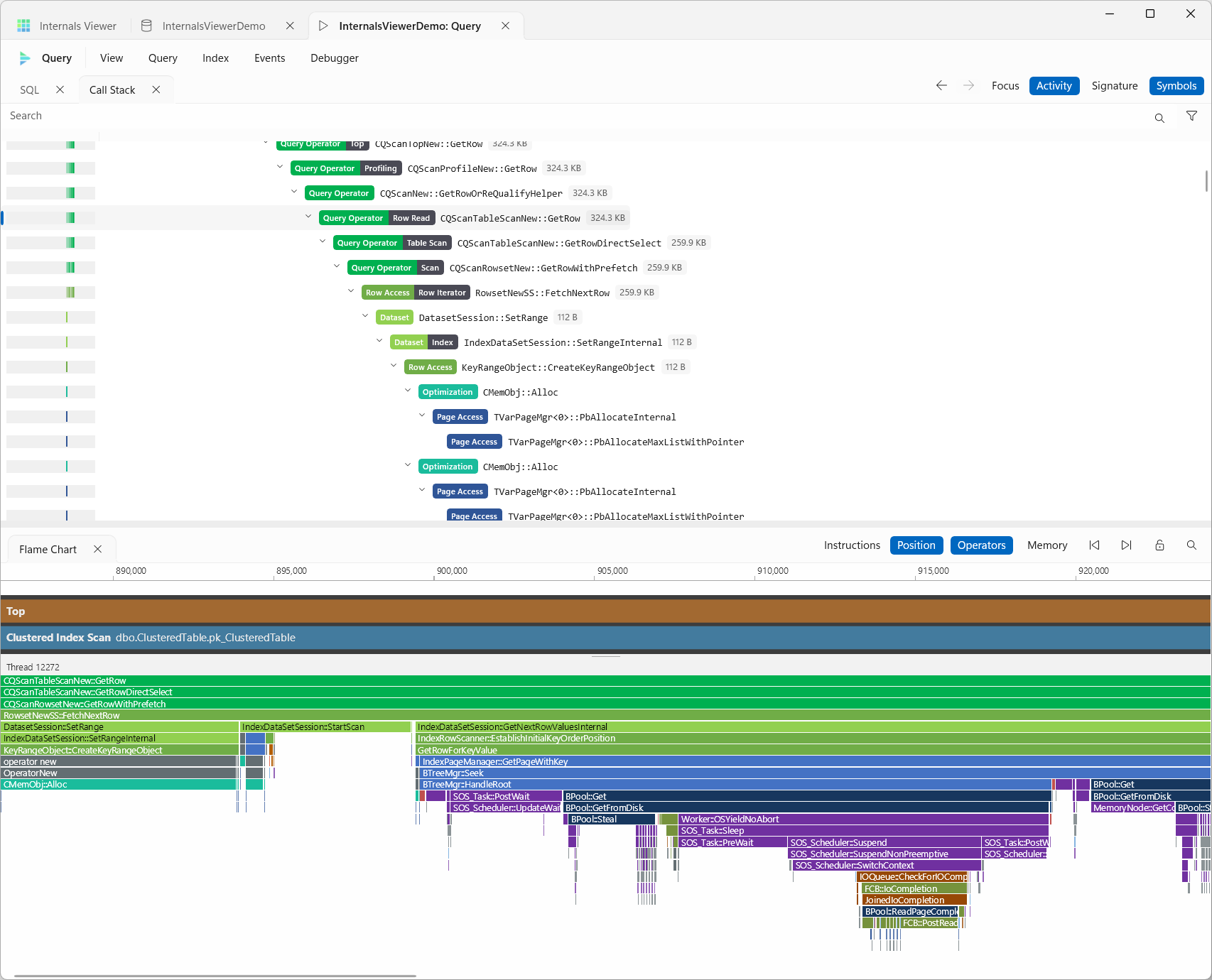
Search

The Search toggle opens a bar above the chart, and Ctrl+F anywhere in the Trace Timeline opens it with the cursor in the box. The strip beneath the ruler, where the playhead's triangle sits, is marked in yellow wherever a call whose function name matches every word typed runs, on any thread, and a yellow bar down the left edge of the Memory History lane marks the rows of each block whose name matches them. A word matches when the name contains it or has its letters in the same order, so qshgr finds CQScanHash::GetRow. Zoomed in, only the blocks alive in the part of the recording on screen are marked. Clicking a yellow bar zooms to what it marks at that point. Over a single call the chart zooms to that call and selects it, and over memory it zooms to the time the blocks there are alive. Hovering over a yellow bar reads Search Results. The number of matching calls and blocks shows beside the box, or No Results when nothing matches. Escape closes it. Right-clicking a function or type name in the Call Stack, its details, the memory Details or a call on the chart gives Search, which opens the bar with that name in it.

Call and Memory after the box choose what is searched, and both start on.

• Call matches calls by function name. A page or row typed as 1:2676 or 1:2676:3, a row id in hex, or rg:1 col:2 for columnstore matches the calls that read it instead, the same as the Call Tree's search.
• Memory matches Memory History blocks by name. An address typed with 0x matches the blocks that contain it, and a page matches the BUFs that held it at any point. While it matches any blocks, the Memory History lane shows only those blocks. With nothing typed, or no block matching, the lane shows every block, objects on the heap first and objects on the stack below them.

As you type, a list under the box shows the matching function names with how many calls each made, then the matching memory blocks with their address and size, each in alphabetical order. Choosing a function or a block puts its name in the box, where it can be edited like anything typed. Open at the right of a block opens it as a memory tab.

The arrows after the box move to the previous or next match in time and bring it into view, and are greyed out while nothing matches. A matching call is selected, and for a matching block the playhead moves to where it was created. Enter in the box moves to the next match and Shift+Enter to the previous one. Stepping starts from the selected call, or from the playhead when nothing is selected.

The filter button beside the Search toggle opens the same category badges as the Call Tree's category filter, beneath the search bar. They are one setting, so hiding a category here hides it in the Call Tree too.

Operators

Operators on the tab strip adds a pane above the threads, with a row per plan operator in the same order and colours as the Timeline's Plan band. A Batch To Row adapter between batch and row mode operators is grey. Each row runs from the operator's first call to its last. The stretches where one of its methods was on the stack are drawn in full colour and the rest shaded, and an operator that ran on several threads gets a track per thread. Either side of that, a fainter bar shows how long the operator's iterator existed. It starts at the iterator's constructor, or for a batch mode operator the call that built it, and ends with the query's CQueryScan::DestroyQuery, where SQL Server frees all of a query's iterators together. When the recording started after an iterator was built, or stopped before the query was torn down, the fainter bar runs to the edge of the recording.

The top row is the statement, such as SELECT, in grey. Its GetRow Returns strip has a tick for each call the statement made to the plan's top operator, with a line down to it, so its Returned ticks are the rows the query returned.

This shows something the lanes cannot. An operator is only on a thread's stack while one of its methods runs, so a Hash Match sits beside its scans in the lanes rather than above them - but its iterator object exists from the moment it is built until the query is torn down, and does its work from its first call to its last. The Operators pane draws both.

• Drag the splitter under the pane to make its rows taller
• Drag the bottom edge of a row to resize that row alone, and the inner edge of a strip to resize that track's strip on every operator. The sizes last until another trace is opened
• Click an operator to select it in the Execution Plan. While Call Stack is off, everything except its calls and the calls beneath them is dimmed
• Double-click an operator to zoom to its lifetime
• Hovering over an operator shows its thread, how many times each of its methods was called, its instructions and positions, the share of its lifetime spent inside its calls (child operators included) and its peak memory in use

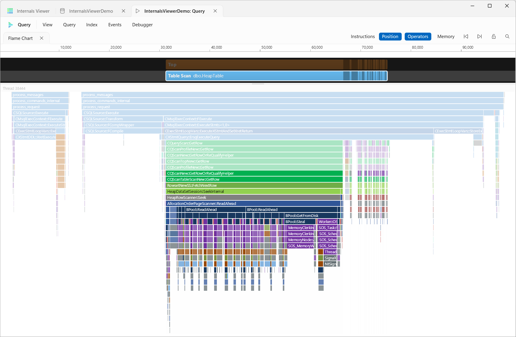
Operator tracks

Each operator bar can carry thin strips of ticks, one strip per track. A tick is one call, drawn as a faint bar across the call with a solid tick at its end. A strip only appears on an operator that has ticks on it, so an operator the track has nothing to say about keeps its full height for its name. Three tracks are built in:

• GetRow/GetBatch - along the top, a tick for every GetRow or GetBatch call the operator answered, coloured by what happened to the row (see below)
• Reads - along the bottom, the operator's requests to the buffer pool
• Evaluations - above the reads, the predicates the operator evaluated

Each track has a toggle under View > Operators, and in the Operators pane's right-click menu. Turning a built-in track off is remembered between sessions.

You can add your own tracks for any function. Add to Operators, in the right-click menu of any call in the chart, adds one for that call's function. Custom..., under View > Operators or in the pane's right-click menu, adds one for a function you pick. A custom track has a tick on the operator each call was made inside, on a lighter strip so it stands apart from the built-in tracks. A call made outside every operator has no tick. The dialog sets:

• Function - the function whose calls are ticked. Type part of its name to pick it from the functions in the trace
• Name - the track's name in the View menu and its tooltips, the function's name to start with
• Colour - the colour of its ticks, the function's category colour to start with
• Height and Width - how tall the strip is and how wide each tick is, as a multiple of the built-in tracks, so 1.5 is half as tall or wide again
• Conditions - which calls get a tick. A call gets a tick only when every condition matches, and with no conditions every call does. Each condition is one of:
  • An argument or the return value, an operator and a value. A number, such as 0, -1 or 0x1F, is compared with the argument's value at its own size. Anything else is compared with the value as the Arguments table shows it, such as true, a page like 1:1536 or NULL.
  • Called By a function, anywhere up the call stack, or Called Directly By a function, the call's immediate caller. The value is a function name, matched the same way as in the Call Tree's search, so *Scan*::GetRow matches any scan's GetRow and sqlmin! limits it to one module. Use != to tick calls that were not made from it.
  • Operator - the operator the tick lands on, such as Filter or Table Scan (Node 3).

For example, CEsExec::FastCompare1 with Called By CQScanTableScanNew::GetRow ticks the predicates a scan evaluated itself, while Operator Filter ticks only a Filter's. A scan below a Filter is also called by the Filter, so Called By the Filter's GetRow would include the scan's too. Use Called Directly By or Operator to pick out the Filter alone.

The same function can be added more than once, such as one track for GetRow calls that returned a row and another for those that did not. Custom tracks last until Internals Viewer is closed, and every trace you open shows them. Turning one off in the View menu hides it like a built-in track. Clear All in the View menu removes every custom track.

Operator Tracks, on the Trace menu, opens a tab listing the custom tracks with their function, conditions, colour, height, width and how many ticks each has in the current trace. Add opens the same dialog, Edit and Delete change or remove a track, and Export and Import save the tracks to a file and load them back, into this or any later session.

• Hovering over a strip names it in a label at the left of the operator, beneath a strip along the top and above one along the bottom, and shows how many ticks of each kind the operator has on that thread
• Hovering over a tick outlines its call in red in the lanes below, and shows what kind of tick it is, its function, thread and position
• Click a tick to select its call in the chart
• Double-click a tick to zoom to it

GetRow returns

A tick is a call to the operator's GetRow, or BpGetNextBatch for a batch mode operator. It ends at the return and is coloured by what happened to the row. Returned rows went on to the operator that asked for them, including every row a blocking operator reads before it returns its first, such as a Sort, an Eager Spool or a Hash Match building its hash table. Skipped rows were taken by the operator that asked for them without it returning a row before it asked again, such as the rows a Stream Aggregate folds into a group. Rejected rows failed a Filter. End is the call that reported there were no more rows.

A line runs from each call up to the operator that made it. The dotted line is the call, in the track's colour. The solid line is the return, in the colour of the call's marker, and meets the marker's edge. The lines are drawn only once the calls are wide enough to tell apart.

Reads

A call to BPool::Get asks for a single page. A call to BPool::ReadAhead asks for a run of pages ahead of the scan. Each read is drawn in the Buffer Pool category's colour, and its tooltip shows the page, or the first page and page count of a read ahead. Pages already in memory and pages read from disk are drawn the same way. The calls beneath a read in the lanes below show which it was, such as BPool::GetFromDisk when the page had to be read. Reads made outside every operator, such as metadata lookups while the query is set up, are not shown.

Evaluations

SQL Server evaluates a predicate with CEsExec::FastCompare or CEsExec::GeneralEval, which write the result into a value passed in by the caller. Each tick is coloured by that result - green for true, red for false and grey for NULL, where a comparison against a NULL could not be decided.

A scan with a predicate pushed down into it evaluates every row it reads but only passes up the rows that match, so the strip shows the rows it skipped as well as the ones it returned. Comparisons an operator makes for its own work are included too, such as a Stream Aggregate checking whether a row starts a new group. Evaluations that produce a value rather than true, false or NULL are not shown, and neither are the three-way comparisons a Merge Join makes between its inputs.

Memory

View > Flame Chart > Memory shows where the query allocated memory, as Allocated or In Use, with None turning it off:

• The memory band - along the bottom of the chart, Allocated is the memory allocated in each sliver of the recording, and In Use is the memory allocated and not yet freed, with its peak in the label. When the plan had a memory grant, the grant is drawn as a box labelled Granted and the line becomes Grant In Use, counting only the query's workspace memory so the two compare like for like. The band needs the Position axis, since each thread counts its instructions separately and they cannot be added together.
• Raised calls - the calls rise off the chart in 3D. A dropdown above the ruler picks Memory: Allocated, which raises each call by the memory it allocated itself, or Memory: In Use, which raises a surface along each call showing what it had allocated and not yet freed as it ran. Hover over a raised call to see its size, and drag one to change the angle and depth of the extrusion.

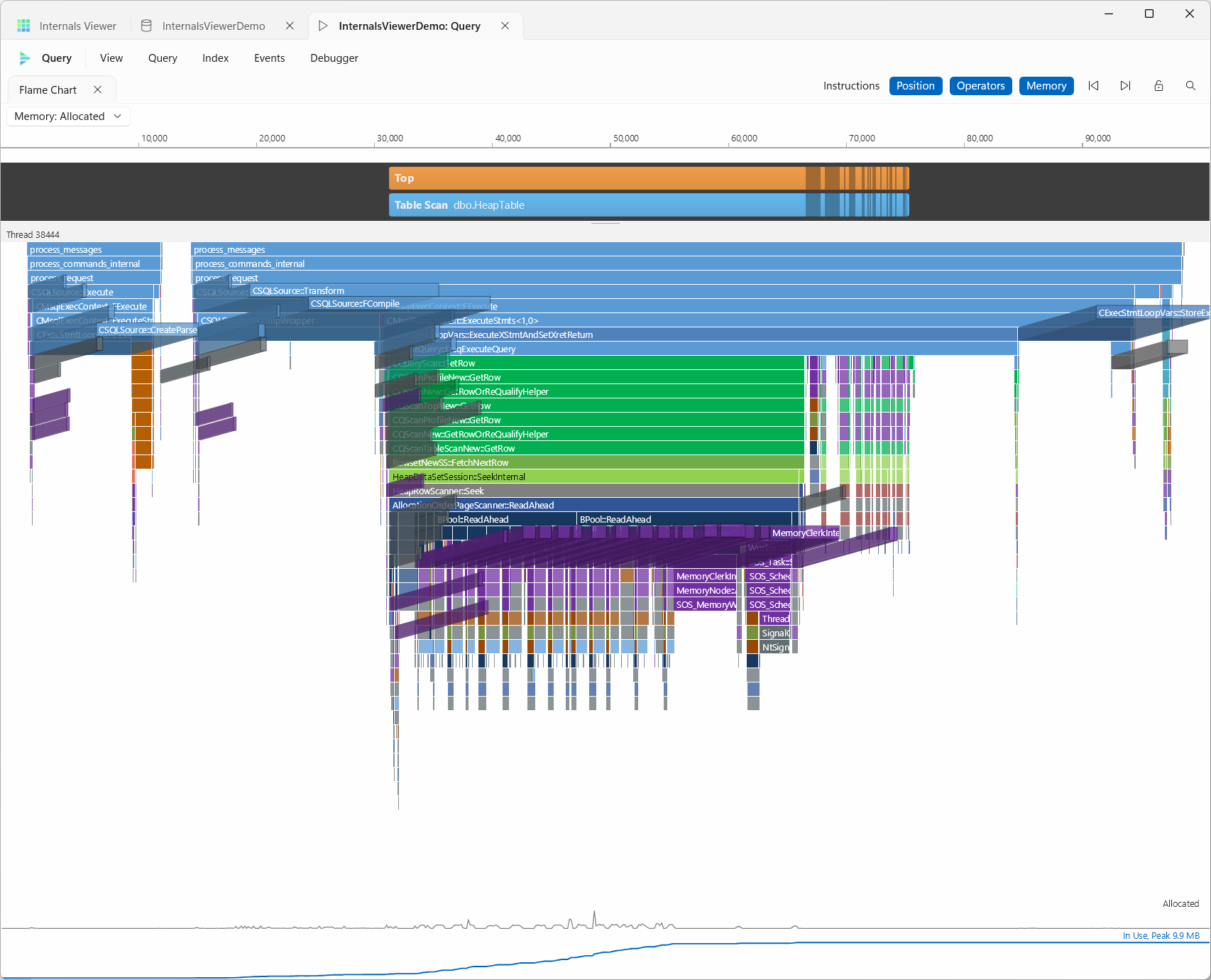
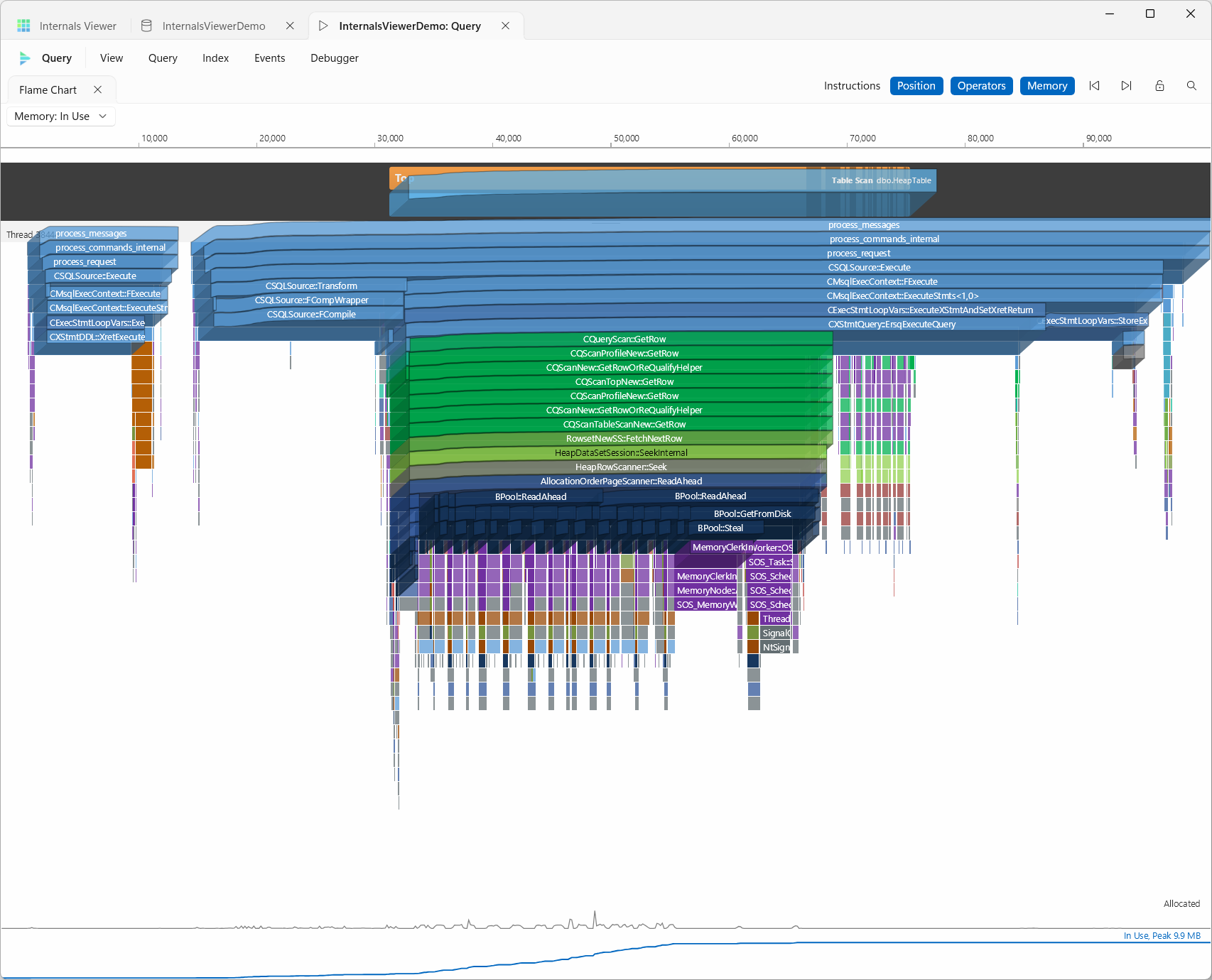
The choice is remembered between sessions, and shared by every Trace Timeline.

Buffer latches

Latching in the Memory History lane's right-click menu, or under View > Memory History, adds a thin row along the bottom of the lane, under a divider, marking every change to the latch of a buffer pool page the query fetched. Each mark is coloured by the latch after the change: blue while it is held shared, red while it is held exclusively, orange while threads are waiting for it, and grey once it is released. Hovering over a mark names the page, such as BUF (1:43), and the latch. Clicking it moves the playhead there and opens the page's BUF, the buffer pool's descriptor for the page, as a memory tab. Latches taken by other threads show on the Position axis only, because the Instructions axis counts the query's own threads. The BUFs themselves are left out of the lane's blocks, and BUF on the same menus adds them back. Both settings are remembered between sessions.

Playhead

Click the ruler or a thread's header to put a playhead on the chart, and drag along either to move it. Its badge gives the position, as sequence:steps on the Position axis. The step back and step forward buttons move it to the start of the previous or next call on any visible thread, and double-clicking the ruler hides it again and clears the selected call and operator.

Trimming the query

Two small handles sit either side of the playhead's triangle, at the bottom of the strip under the ruler. Drag one away from the playhead to trim the query to the stretch between them, and drag either again to move that end. Outside the trim is shaded and the playhead stays inside it, but the chart keeps its zoom. Memory History, the Memory History lane, the latch row and search then count only what happened inside the trim. Memory History and its lane keep every block the query created that changed inside the trim, even one created before it, and a reference graph is drawn from the pointers held inside it and counts only the changes made inside it, so Reference Changes and Data Changes show what was busy in that stretch. The Operators lane is not trimmed, and pointers still resolve against the whole recording. Double-click the playhead's triangle to remove the trim.

Play moves the playhead steadily along the chart, scrolling the view on when it reaches the edge, and stops at the end of the recording. With the query trimmed it plays the trimmed stretch over and over until you pause it. It starts from the playhead, or from the left of the view when there is none or the playhead is already at the end. Click it again to pause.

With the memory view set to None and Call Stack off, the calls under the playhead pop out of the chart, each raised by the memory it allocated, so scrubbing along shows which part of the stack is allocating. Drag a raised call to change the angle and depth, as with the memory view. With a memory view on, the band marks the memory allocated and in use at the playhead.

How this works

Each bar is one call recorded during the Full Trace replay, with where it started and ended in the recording, the instructions it executed, its thread and its place in the call tree. Positions are shared by every thread, which is why that axis lines them up, while each thread counts its own instructions.

See How Full Trace works for the details.

Call Stack

View > Call Stack, or Call Stack at the bottom of the right-click menu, opens a tab beneath the chart listing the calls that led to the selected call. With nothing selected the tab reads No Call Selected. Its tab strip has the Decode toggle and step back and step forward buttons, which select the previous or next call at the same depth as Left and Right do. The stack sits under a row for the selected call's thread, each call shown as the function's signature with each parameter's type and the value it was passed, coloured as in the Call Tree's signatures. A dot before each call shows its category's colour, and hovering over it names the category. A value that decodes to an object shows the object's class instead of its declared type. this is shown without its address, unless it decodes to something such as an operator or an index, and its address is in the call's details. The innermost call comes first, highlighted and marked with a red arrow, and each call below it is the one that called it, as a debugger lists a stack. The pane selects the same call as the chart, and opens its details beside the stack. The values decode as they do in Arguments, and the Decode setting is shared. Drag the tab to dock it above, below or beside the chart, and drag the splitter between them to resize it. Its X, or turning Call Stack off, closes it.

A value that points into memory the trace recorded has a Show Memory button, which opens that block's bytes as a tab of its own, named after the object. Right-clicking such a value, in a call's signature or in its details, offers Memory History, which opens the same tab at the address it points to, including a value already shown as the object it points into. A value that points into a buffer pool page reads Buffer Pool Frame: with the page the frame held at that moment and how far into the page it points, such as Buffer Pool Frame: (1:100) +0x1A0, and the same goes for pointers in a memory tab's Writes and in a batch's fields. A pointer to the BUF, the buffer pool's descriptor for the page, reads Buffer Pool: (1:100) BUF and opens the page without selecting a record. Clicking it opens the page with the record holding that byte selected. The page opens as it is now, not as it was during the query. A page from another database, such as tempdb, is named with its database and does not open. Its tab strip has step back and step forward buttons, which select the previous or next write in the Writes list, so the playhead and the outline follow it. With a filter set they step through the writes the list shows. Clicking a block in the chart's memory lane opens the same tab. When the value points inside the block, or the click was part way along it, the bytes scroll to that address and it is outlined. Each block gets one tab, and its bytes follow the playhead, with the bytes each call changed marked in the call's category colour. An 8-byte value in the bytes that points into recorded memory or into a buffer pool page is underlined and drawn in grey, since it is an address rather than a value to decode. Hovering over it names what it points to, and Ctrl+Click, or Open Memory or Open Page on the right-click menu, follows it. Memory tabs dock and resize like the Call Stack, so they can share its tab strip or sit on another side of the chart.

While a memory tab is the one showing, the strip beneath the ruler is marked where that block was written, each mark in the colour of the writer's category, so you can see when it changes. Hovering over a mark reads the tab's name followed by Updates, and clicking there moves the playhead to it. With a search open as well, the search marks take the top half of the strip and the memory marks the bottom half. Widen a memory tab and its tabs appear beside the bytes. Details gives the block's address, marked Heap or Stack, its type and length, its lifetime as the positions it was created and destroyed at, the function that created it, how many updates it had, and the functions that wrote to it with how many writes each made, coloured by category and listed in the order they first wrote. For an object on the stack the lifetime runs from the first call that held it to the end of the last, followed by how many instances it had, and the function that created it is the one whose stack holds it. It has no Reads or Read By, because reads are only recorded for heap memory. It also gives how many times the block was read, and under Read By the functions that read it with how many reads each made, in the lighter shade of their category colour. Writes lists every write to the block with its position, function, address, length and value. The value is the bytes written as hex, or decoded as the type of a watch pinned on those bytes. Clicking a write moves the playhead to it, scrolls the bytes into view and outlines them, and the pin at the end of a write adds a watch on those bytes. The Function and Address boxes filter the list, Show Writes on a function's right-click menu in Details or clicking a byte in the hex fills them in, and right-clicking a write offers Filter To Function and Filter To Address. The position, address and value columns sort when their headers are clicked. Reads lists each call that read the block, with the position of its first read, the function, the call, the address and length of the bytes it read, and how many reads it made. A call that reads several fields is one row covering all of them. Its function is shown in a lighter shade of its category colour, and the list filters, sorts and outlines the bytes read the same way. Show Reads on a function's right-click menu under Read By fills in its Function box. Watches lists the pinned watches with an editable label, the type the value is decoded as and its value at the playhead, and a button to clear each one. References lists the 8-byte values in the block that point into recorded memory or into a buffer pool page, each with its offset, the address it holds and what it points to, so two pointers to objects of the same type can be told apart. The box above the list filters it to the pointers whose target or address contains what is typed. Expanding a pointer lists the pointers found from the address it points to, read at the playhead, so a chain of structures can be followed as far as it goes. A pointer into the middle of a block, including one into the tab's own block, lists the pointers from that address to the end of the block, with offsets counted from that address. Collapsing a pointer and expanding it again reads it afresh. A pointer to an address already followed on the path, or to the start of the tab's own block, is marked (Cycle) and can still be expanded. A pointer whose target has changed since the pointer was written is left out, here and in the underlines in the bytes. An example is a pointer a compiled plan keeps into compile memory that was freed and has since been reused for a page. Graph beside that box, Open Reference Graph on a memory tab's right-click menu, or right-clicking a block in the Memory History lane opens the block's pointers as a graph in a query tab of its own, docked along the bottom of the query so the Trace Timeline stays in view while the graph follows the playhead. It can be dragged elsewhere like any other tab, and a second graph opens beside the first. Along its top the graph's name is followed by how many objects it shows, with a spinner while it is being worked out, and a search box on the right lists the boxes whose names or addresses match. Choosing one scrolls the graph to its box and outlines it. Object Graph, on the Trace menu, opens a graph that starts from a call rather than a block: the first call on the Trace Timeline, which with Crop To Query on is the start of the query itself. Its first box names that call's function, and its connectors lead to the objects the call was given, each labelled this or with the register or stack location the argument was passed in, such as RDX. From there it reads like any other graph. The graph is drawn from every pointer the block's fields held across the recording, or across the trim, so its shape stays put while the playhead moves and only the values in its boxes change. Each field that held a pointer is a box naming the type it points to, with the address it holds at the playhead beneath, and each buffer pool page is a shaded box naming the page. A box shows the object as a whole, and where in it a pointer lands is written on the pointer's connector. A scan's array of column bindings is the exception: expanding it shows each binding as a box of its own, ColumnBinding[0], ColumnBinding[1] and so on, each with the pointers it holds. A box whose object has watches pinned on it lists them under its address, each with its label, or its offset and type when it has none, and its value at the playhead decoded the same way as on the memory tab's Watches. A column binding's box lists only the watches that fall inside that binding. A field that is empty at the playhead keeps its box, with its name greyed out and no value, because it is not set yet, has been cleared, or what it pointed to has been freed. A box that only ever holds one object shows that object for its whole life, from allocation to free, even before anything on the path points at it, so you can open it whenever it exists. A page used by a sort or a workfile is named Sort Page or Workfile Page. A field that pointed to objects of different types names them all, separated by a slash, until the playhead reaches one of them. A BUF whose frame was set before the recording, because its page was already in the buffer pool, still points to its frame, taken from where the query found the page. A field that moves from object to object, such as the BUF of the page being scanned, is one box whose value changes as the playhead moves, and the fields under it follow whichever object it points to at the playhead, so the frame under a BUF changes with it. The tab's own block starts expanded, and the arrow at the right of any other box expands it to show its fields, or collapses it again. A box whose objects never held a pointer has no arrow. Right-clicking a box offers Expand All, which expands it and everything under it, and Collapse All, which collapses it and everything under it and closes the objects on its left. Right-clicking the first box does this for the whole graph. Neither is available while Reference Changes or Data Changes is on, as those already expand as far as they need to. Select on a box's right-click menu starts the graph again from that box's object, the one it holds at the playhead, and the graph's title follows it. Reset, on the right-click menu of the graph's background, goes back to the object or call the graph was opened on. A very large graph stops growing once it reaches its limit, which the count along its top notes, and it fills each column before starting the next, so what it leaves out is furthest from the start. Each pointer is a stepped connector with the field it is held in written above it, and the offset it lands at when that isn't the start. A field that moves around inside the same object, such as a pointer stepping through the rows of a page, shows the offset it points to at the playhead, so the label changes as the playhead moves. A connector whose pointer went on to point somewhere else is drawn in orange, with how many times it did beneath it. Only moves you would see in the box count, so a move made while the path led to a different object is left out. Only a move from one place to a different one counts. Clearing the field, setting it back to the same place, and pointing it back into its own object, as an empty list does, are not changes. The call that first sets a field is setting it up, so none of its writes to that field count, however many it makes. After that every move counts, including several within one call. Nothing from the start of the query's shutdown onwards is counted. When an object holds several pointers into one other object, each field gets its own connector, labelled with the field and where in the other object it points, and they fan out and collect back into that object's single box like the rungs of a ladder, starting below the box so the first does not look like a direct connection. Several dashed links, or links on the left, from one object to another share a connector instead, labelled with the first and how many there are, and hovering over the connector lists them all. A pointer to objects already on the graph, by another path or round a cycle, is a dashed connector to the box that shows them rather than a second box, so the graph stops there. That holds wherever in the object the pointer lands, and a box shows the object's own address. Dashed connectors are drawn lighter than solid ones, and run on their own verticals between a box and its solid connectors, so they never lie on top of a solid one. One going down leaves below the middle of its box and arrives above the middle of its target. One going up leaves above and arrives below, and turns closer to the box. One that would have to cross a column of boxes to reach its target runs along the gap between two rows instead, so it never passes behind a box. A dashed connector's label is only written, beside the box it leaves, while the pointer is over the connector. Labels on solid connectors that would land on top of each other are stacked. Hovering over any connector, or its label, draws it in green on top of the others, and its tooltip names the boxes at either end, the field and how many changes it had. Reference Changes and Data Changes on the graph's tab strip narrow the graph to what changed, expanding as far as they need to, with the objects on the shortest way to each. Only one can be on at a time, and with neither on the graph shows everything you have expanded. Reference Changes shows the pointers that changed. Data Changes shows the objects whose other fields changed after the call that set them up and before shutdown, leaving out the last call when it clears a field for good, and hovering over a box's name gives how many data changes it had. A field whose objects are all already on the graph is left out, along with the path to it, so if an object and one of its fields both point to the same BUF only the object's own pointer is drawn. The dashed connectors are left out too. The arrow at the left of any box shows the objects that point to it in the column to its left, and the same arrow on each of those shows the objects that point to them, further left. For a box out on the right of the graph they start on the row below it, and their connectors arrive below the middle of the box, so they stay clear of the connector from the box's own parent. The arrow is only there when something not already on the graph points to the box. Each connector on that side carries its label beside the object it comes from, since several objects can point into the same box. An object already on the graph is not added again, so the graph never loops back on itself. Objects allocated in the same place that point to it at different times share a box, which shows whichever one points to it at the playhead. The mouse wheel scrolls the graph, Shift + the mouse wheel scrolls it sideways, and dragging its background moves it. Ctrl + the mouse wheel zooms in and out at the pointer, and Shift + drag draws a rectangle and zooms to it. Right-clicking the graph, or a box, offers Zoom to 100% and Zoom to Fit. Zoomed out too far to read the detail, each box shows only its name, written larger, and the connector labels and the band along the top are hidden. While the labels are readable, a thin band along the top of each box is a small timeline of the recording, or of the trim. A thin line under the band is the lifetime of the object the box shows, from when it was allocated to when it was freed, over a light track that runs the width of the band. The line is in the colour of the category of the function that allocated the object, or darker grey for a page or an object whose function has no category. It is marked wherever the box moves to point somewhere else, and wherever the object's other fields change, each mark in the colour of the category of the function that wrote it, with nothing marked from the start of shutdown. It is shaded grey up to the playhead, so you can see how far the playhead is from the next change. Clicking a box's name opens what it points to at the playhead as a memory tab, or opens the page. Hovering over a box outlines the object it shows at the playhead in the Memory History lane, the same outline as hovering over the lane itself, and scrolls the lane to it when it is out of view. When the playhead is outside the box's lifetime it outlines the object the box last held, or the first it will hold if the playhead is before them all. Clicking a target opens it as a memory tab or opens the page, and selecting a pointer at the top level outlines its bytes. Every BUF the query fetched is recorded too, named after the page it held, such as BUF (1:43), and its memory tab has a BUF tab as well. It names the page the BUF holds at the playhead, which opens it, and reads its frame address and its latch: held shared and by how many, held exclusively or released, whether threads are waiting, the latch's owner and waiter list, and the raw state. The bindings a scan uses to copy each row into its row buffer have a Bindings tab. On the bindings object it gives the number of columns and a link to the column bindings. On the column bindings, and on the row buffer itself, it lists each bound column with its ordinal, type and size, where it sits in the record (or Variable and its number among the variable columns), where its status, length and value go in the row buffer, its flags with Length shown when the length is written separately and By Reference when the value is a pointer rather than a copy, and a link to its Column Attributes. A colour key in a heading shows the colour that field is marked in. Selecting a column marks its bytes in those colours: every field of its column binding, or its status, length and value in the row buffer. Links along the top open the bindings object, its column bindings and the row buffer. It also gives the BUF's database ID, partition, status, error code, state history, read time in microseconds, when it was last used and recovery unit. While the tab is selected those fields are marked in the bytes. A field that DBCC PAGE prints in its BUF section carries that name too, such as Status (bstat). Positions are shown as sequence and step in hex, and every position is a link that moves the playhead there. Clicking a function in Details moves the playhead to its first write, or under Read By its first read. Right-clicking a position or a function in Details gives Zoom to, which zooms to the call and selects it, and Call Stack, which moves the playhead there and opens the Call Stack. A function also gives Find, which finds the call in the Call Tree. For a function that wrote or read more than once these act on its first write or read and read Zoom to First and Call Stack First. Right-clicking the address gives Find, which finds the calls that used it. Hovering over a position marks it on the chart and shows the chart's map of the whole recording with the position on it, and hovering over a function in Details highlights its writes, or under Read By its reads, in the lanes.

Selecting a call further up the stack, with Up or by clicking it in the pane, keeps the stack as it is and moves the selection along it, so Down comes back the same way. Selecting a call that is not on the stack, by clicking its bar or with Left and Right, starts a new stack ending at that call. The pane follows the category filter and Scope, so its calls are the ones drawn in the chart above it.

Clicking a call selects it in the chart, the Call Tree and Arguments, the same as clicking its bar, and opens its details beside the stack. These show its category, its module, this and the value it returns. They also show its Call Id, the number that Source shows in brackets, the trace positions it started and ended at, how many instructions it executed, and its Arguments, each with its number, type and value. Clicking an argument shows that value's details, as clicking it in the stack does. Right-clicking a call gives Open In Call Tree, Zoom, which fits the chart to that call, Scope, which scopes the chart to its function the same as the chart's own Scope, Copy Signature, which copies the line as it reads, with its types and values, Copy Symbol, which copies the function's name, and Copy Address, which copies the function's address. The copy button at the end of each call copies its signature, and every value in the details has a copy button beside it too. The value a call returned is in its details rather than the stack. The details are headed by the function's name. Clicking a value shows its details in place of the function's, and adds its argument number and type to the heading, such as [3] SEBindings const *. Right-clicking a value gives Copy Decoded, Copy Value and Find. In the details, the positions the call started and ended at are links that move the playhead there, and right-clicking one gives Zoom to and Call Stack. Right-clicking this, the value returned or a selected value gives Find when it is an address. The selected call's function, or the selected value, is highlighted in the stack in the same way as a search match, until the details are closed.

An object's details end with its Source, the path that brought it to the call, when there is one to trace. Each step, a little further in than the last, is a call further up the stack that was passed it too, and the path ends at the call that created it, marked with a green plus, such as its constructor or the allocation it was made in. Each step shows its call's number in the trace in brackets, so the numbers fall as the path goes back in time. A step that is not on the stack in the pane, such as a constructor that has already returned, opens to list the stack at that call, the function's callers in order, innermost first. An object that was in use before the trace began ends at the first call seen using it, without a plus.

Hovering over a step, or over a function listed under an opened step, highlights it and marks where its call starts with a green line from the call's bar down to the bottom of the chart. When the chart is not showing the call, because it is outside the part in view or outside the chart's scope or filter, a small map of the whole trace appears in the corner instead. It shows the step's call as a black line from its depth down, with the playhead in red when there is one, and the part in view shaded, so you can see how far away it is. When the chart is scoped, only the scope's calls in view are shaded. The map includes calls that the chart is hiding. Right-clicking a step, or a function listed under an opened step, gives Go To, which moves the playhead to the start of its call. If the call is outside the chart's scope, the scope is cleared first.